Analysis of Pre- and Post-Test Data from the CC Cert Course, January 2022
Updated June 2022

Background

In mid-2020, a large bank of very specific, technical questions on the material in the Creative Commons Certificate course was developed. CC General Counsel Sarah Pearson, Assistant Direct of Open Education (at that time; now: Director of Learning and Training) Jennryn Wetzler, and long-time Certificate course facilitator Jonathan Poritz painstakingly wordsmithed the language of the questions, made sure they were legally precise, and chose a set covering the core of the material the cert course seeks to impart to its graduates.

This work lead to an online quiz administered as a Google Form, which seems to take folks about 35 minutes to complete and has a maximum score of 60 points (roughly, but not exactly, one point per question: some questions have several parts and so are worth several points).

Since the survey instrument was finalized, it has been offered to participants before and after they take the course. They are asked if they would be willing to volunteer their time to take the survey. They are also told that the survey results will have no impact on whether they pass the course or not, and that its only purpose is to help us improve the course.

After a first dataset was collected with this survey, an analysis was performed and the results are given in the page Some Pre- and Post-Test Data from The CC Cert Course, December 2020.

This page instead shows the results of an analysis of all of the data collected through 17 January 2022. That dataset included 277 instances of the test being taken, being 203 from before the participant took the course and 74 from after. Test takers were from all three flavors of the cert course available up to now, being Educator, Librarian, and GLAM — although the GLAM version is only recently available and so there are quite few test instances from those participants.

Update Background:

This page was slightly updated in June of 2022. The changes were:

  1. A new version of the script which makes the graphs was created
  2. The command lines for each graph, using the new script, were noted with each graph.
  3. A section of additional graphs was added, showing unit-level performance.

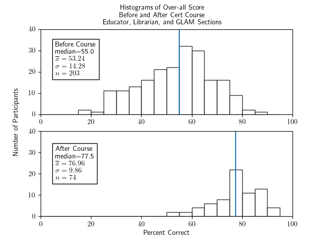
First, the over-all pre- vs post-test scores for all participants:

Total Score, All Participants, Pre- and Post-Test:
 
   Two histograms of percentage correct of the whole test for all cert participants - Librarian, Educator, and section - one histogram for before the course and one for after.  Both show fairly symmetric and roughly bell-shaped distributions.  The histogram for before the course has a median of 55.0, an x-bar of 53.24, a sigma of 14.28, and an n of 203.  The histogram for after the course has a median of 77.5, x-bar=76.96, sigma=9.86, and n=74.
 

  1. If you're a little rusty in your statistical terminology:
    1. These are histograms, meaning that the heights of the bars indicate how many scores lie in the range of percentages covered by the base of that bar on the horizontal, "Percent Correct," axis. For example, the bar in the "Before Course" histogram whose left edge is at location 60 on the horizontal axis has base going from 60 to 65 on that horizontal axis and height of 13. That means that 13 participants' pre-test scores were in the range 60 to 65% correct.
    2. The vertical blue line in these histograms is located at the median of the scores for that graph, meaning that half of the scores in that dataset are less than (to the left of) that score, and half are greater than (to the right of) that score: it is a good measure of the "middle value" of the dataset.
    3. The $\bar{x}$ in the key box in each graph indicates the mean (or average) of that dataset, which is another measure of the middle of data, but means are more sensitive than medians to outliers, meaning that atypical scores way off to one end will pull the mean in that direction but not the median.
    4. The $\sigma$ in the box is the standard deviation of that dataset, which is a measure of how much variation there is in the data.
    5. The $n$ in the box tells the size of that dataset.
  2. This graph was produced with the command
    ./make_graphs.py --prepostall --allsections --ylim 40
    as described in the below section How were these graphs made?.

We can summarize this by saying

We have statistically significant evidence that the post-test scores are more than 21.2% higher than the pre-test scores, at the 5% significance level.


Disaggregating by version — Educator/Librarian/GLAM — of the cert course.

If we consider only participants who took the Educator section, we have these paired histograms:

Total Score, Educator Sections Only, Pre- and Post-Test:
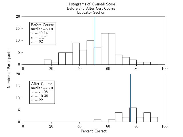
 
   Two histograms of percentage correct of the whole test for participants in the educator section only - one histogram for before the course and one for after.  Both show fairly symmetric and roughly bell-shaped distributions.  The histogram for before the course has a median of 50.8, an x-bar of 50.14, a sigma of 14.7, and an n of 82.  The histogram for after the course has a median of 75.8, x-bar=75.98, sigma=10.38, and n=22.
 

  1. Same statistical terminology reminders above apply here as well.
  2. While the sample sizes are smaller than the entire set of folks who took the survey, they are still large enough that it is comfortable to draw statistical conclusions.
  3. This graph was produced with the command
    ./make_graphs.py --prepostall --ed --ylim 20
    as described in the below section How were these graphs made?.


Now looking only at participants who took the librarian section, we have these paired histograms:

Total Score, Librarian Sections Only, Pre- and Post-Test:
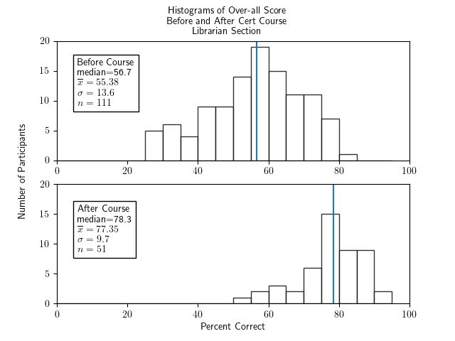
 
   Two histograms of percentage correct of the whole test for participants in the librarian section only - one histogram for before the course and one for after.  Both show fairly symmetric and roughly bell-shaped distributions.  The histogram for before the course has a median of 56.7, an x-bar of 55.38, a sigma of 13.6, and an n of 111.  The histogram for after the course has a median of 78.3, x-bar=77.35, sigma=9.7, and n=51.
 

  1. Same statistical terminology reminders above apply here as well.
  2. Again, sample sizes are fine.
  3. This graph was produced with the command
    ./make_graphs.py --prepostpass --lib --ylim 20
    as described in the below section How were these graphs made?.


We have a bit of a problem with the GLAM section, though, because it was so new when these data were collected and so we have only one post-test, and a very statistically uncomfortable ten pre-tests. That means that we should not draw any conclusions from the following histograms, although we include them here for completeness.

Total Score, GLAM Sections Only, Pre- and Post-Test:
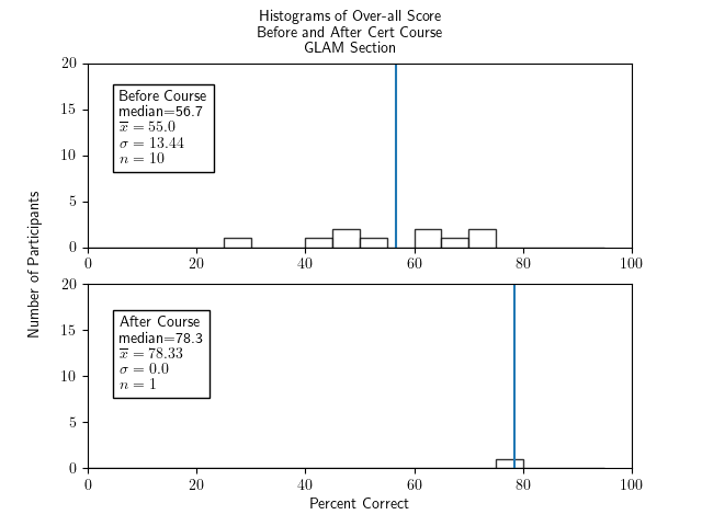
 
   Two histograms of percentage correct of the whole test for participants in the GLAM section only - one histogram for before the course and one for after.  Both show fairly symmetric and roughly bell-shaped distributions.  The histogram for before the course has a median of 56.7, an x-bar of 55.0, a sigma of 13.44, and an n of 10.  The histogram for after the course has one value, at 78.3.
 

  1. Same statistical terminology reminders above apply here as well.
  2. This graph was produced with the command
    ./make_graphs.py --prepostall --glam --ylim 20
    as described in the below section How were these graphs made?.


We can summarize this by saying that, excluding the GLAM sections because we don't have enough data, both the educator and librarian participants had fairly similar starting scores, ending scores, and (therefore) gains from taking the course as each other (and the whole group).

Possible sources of bias in this study, and an answer to one such

Those of us who love nothing more than to analyze a little data and try to learn from it, and who have experience doing so, will have one huge concern about the discussion above: while the samples (except for the one from GLAM participants) were of reasonable size, the were all volunteers! This means we are in serious danger of volunteer sample bias.

Volunteer sample bias is when some characteristic (called a "lurking variable") determines (or elevates) participation in the study which also affects the way people respond to the survey questions themselves. For example, in many classroom situations, if there is a voluntary survey at the end of the course, only students who feel particularly strongly about the course — either they loved it or hated it — will bother to do the survey; the lurking variable here is "how strongly do students feel about the course." This is why the histogram showing "over-all teaching quality" for a volunteer survey administered after a class is over often does not have a classic bell ("normal" is the technical term) shape, but rather has a bimodal (two peaked) shape.

We don't really have a option to force folks to take the survey (nor would it be ethical to do so) before or after the cert course. So we will always have to deal with some level of volunteer sample bias.

But we can rule out one particular mechanism for this bias! One might fear that only folks who did well in the course would feel good enough about the course to volunteer to take the post-test. This is like the bimodal love/hate survey results mentioned above, except that since the survey doesn't give haters the chance to down-score the course as a whole, they are probably unlikely to bother to take the survey after finishing the cert. We're basically worried here that there is an artificial mechanism which would result in a bimodal distribution but cuts off the lower peak, so we're spuriously seeing just the higher peak.

We have enough information to figure out for each time the cert survey was taken if that person would go on to pass the course, if they were taking it before the course, or if they did pass the course, if they were taking it after the course.

At first it seems as we feared, that only the successful students bother to take the post-test: of the $n=74$ post-test scores shown in the first pair of graphs, above, a full $73$ of them were folks who went on to pass the course! It would be possible, then, that the participants get nothing out of the course at all, but the difference shown above between pre-test and post-test scores is simply due to that fact that the pre-test data includes both folks who do already know the material and those who don't, and the post-test appears to show improvement simply because it doesn't have any data for the folks who didn't start out knowing everything.

In fact, here's a graph which seems to support this possible source of bias:

Pre-test Score, All Participants, Broken Down By Eventual Fail or Pass:
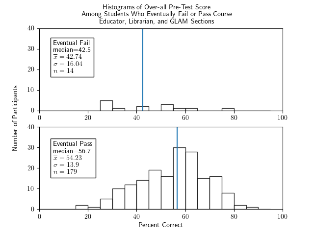
 
   Two histograms of percentage correct of the pretest for all cert participants - Librarian, Educator, and section - one histogram for those who eventually fail, one for those who eventually pass. The graph for failed students shows an amorphous, largely flat graph with median of 42.5, an x-bar of 42.74, a sigma of 16.04, and an n of 14. The graph of passing students shows a fairly symmetric and roughly bell-shaped distribution with a median of 56.7, an x-bar of 54.22, a sigma of 13.9, and an n of 179.
 

  1. Same statistical terminology reminders above apply here as well.
  2. This graph was produced with the command
    ./make_graphs.py --pretestpassfail --allsections --ylim 40
    as described in the below section How were these graphs made?.

In essence, we might worry that the difference between the pre-test and post-test populations is simply that the pre-test has a mixture of good and bad students while the post-test is only the good students: i.e., maybe the course doesn't teach anything, but merely convinces the bad students not to take the post-test, so the distribution of post-test scores of course looks better than the distribution of pre-test scores.

But we can rule out that depressing possibility. If it were true, then when we make a pair of histograms for over-all score before and after the course of only participants who were successful in the course, then they should look pretty much the same!

Instead, here is that pair of histograms:

Total Score, Successful Course Participants Only, Pre- and Post-Test:
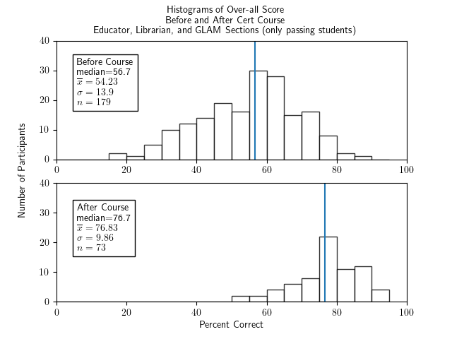
 
   Two histograms of percentage correct of the whole test for cert participants who passed the course and were in any section - Librarian, Educator, and section - one histogram for before the course and one for after.  Both show fairly symmetric and roughly bell-shaped distributions.  The histogram for before the course has a median of 55.0, an x-bar of 53.24, a sigma of 14.28, and an n of 203.  The histogram for after the course has a median of 77.5, x-bar=76.96, sigma=9.86, and n=74.
 

  1. Same statistical terminology reminders above apply here as well.
  2. This graph was produced with the command
    ./make_graphs.py --prepostpass --allsections --ylim 40
    as described in the below section How were these graphs made?.

The fact that this pair of graphs is so similar to the first graph on this page is strong evidence against the previously stated, unfortunate hypothesis about how voluntary survey participation might give misleading conclusions, and is evidence that taking the course does result in, on the average, more than 20% increase in performance on the core knowledge test.

For completeness, let's make the same paired graphs for the individual flavors of the course, just to answer any potential fear that the ugly hypothesis "the course merely filters out the poorer students and doesn't teach anything, looking only at the Educator/Librarian/GLAM version."

Total Score, Successful Educator Course Participants Only, Pre- and Post-Test:
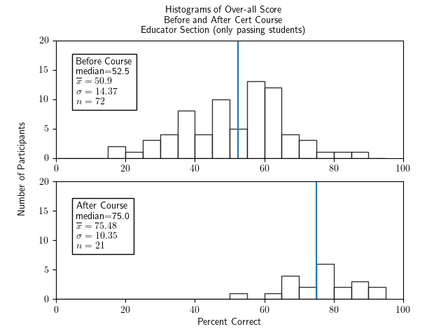
 
   Two histograms of percentage correct of the whole test for cert participants who passed the course and were in Educator section, one histogram for before the course and one for after.  Both show fairly symmetric and roughly bell-shaped distributions.  The histogram for before the course has a median of 55.0, an x-bar of 53.24, a sigma of 14.28, and an n of 203.  The histogram for after the course has a median of 77.5, x-bar=76.96, sigma=9.86, and n=74.
 

Total Score, Successful Librarian Course Participants Only, Pre- and Post-Test:
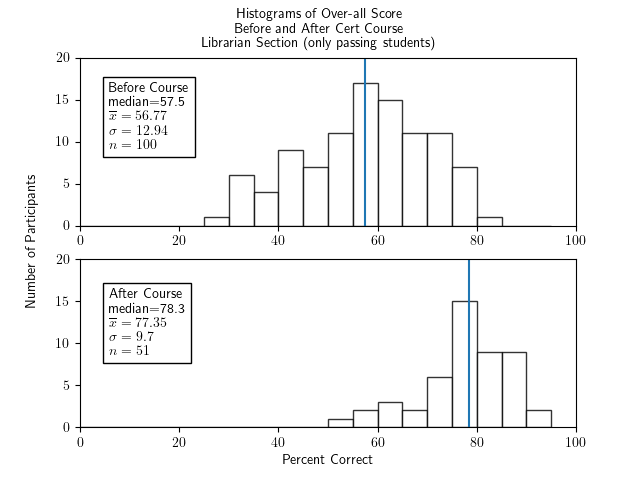
 
   Two histograms of percentage correct of the whole test for cert participants who passed the course and were in Librarian section, one histogram for before the course and one for after.  Both show fairly symmetric and roughly bell-shaped distributions.  The histogram for before the course has a median of 55.0, an x-bar of 53.24, a sigma of 14.28, and an n of 203.  The histogram for after the course has a median of 77.5, x-bar=76.96, sigma=9.86, and n=74.
 

Total Score, Successful GLAM Course Participants Only, Pre- and Post-Test:
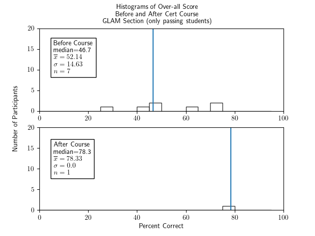
 
   Two histograms of percentage correct of the whole test for cert participants who passed the course and were in GLAM section, one histogram for before the course and one for after.  Both show fairly symmetric and roughly bell-shaped distributions.  The histogram for before the course has a median of 55.0, an x-bar of 53.24, a sigma of 14.28, and an n of 203.  The histogram for after the course has a median of 77.5, x-bar=76.96, sigma=9.86, and n=74.
 

  1. As before, the sizes of these restricted samples are still quite reasonable, with the exception of GLAM because it had just started when these surveys were conducted. We should, therefore, not try to draw any strong conclusions for the GLAM section and only include its graph for fun (and maybe because we're a little obsessed...).
  2. The first of these three graphs was produced with the command
    ./make_graphs.py --prepostpass --ed --ylim 20
  3. ...the second of these three graphs was produced with the command
    ./make_graphs.py --prepostpass --lib --ylim 20
  4. ...and the third of these three graphs was produced with the command
    ./make_graphs.py --prepostpass --glam --ylim 20
    as described in the below section How were these graphs made?.

These pairs of graphs are also very similar to the earlier ones, which can be taken as strong evidence against the previously stated, scary hypothesis about how voluntary survey participation might give misleading conclusions, and is more evidence that taking the course does result in, on the average, more than 20% increase in performance on the core knowledge test.

Unit-level performance

The questions in the survey instrument can be classified by the course unit to which they correspond. It might thus be interesting to see the pre- and post-test performance on each unit, both for all students in one graph and also disaggregated by which section of the course the student was taking. (The section presumably tells the background of the student: most (but not all) of the folks in the Librarian section were librarians, etc.) Each graph is followed by the script command which made it, as described in the below section How were these graphs made?.

Unit 1: What is Creative Commons?

7 of the 60 survey points, or 11.6%, were on material from Unit 1.

Unit 1 Score, All Participants, Pre- and Post-Test:
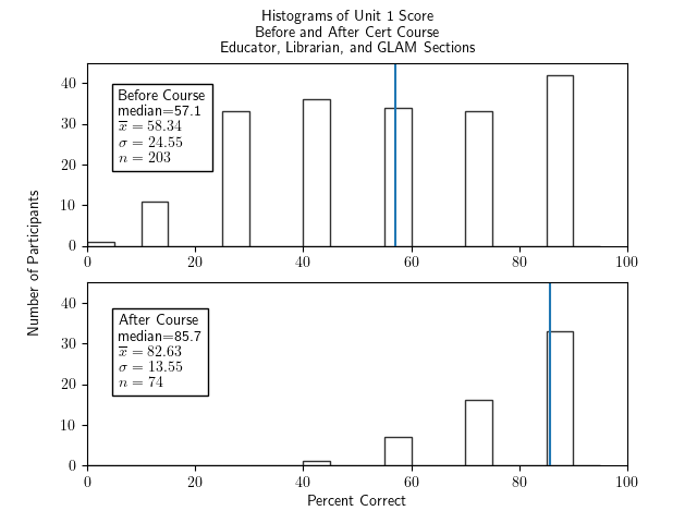
 
   Two histograms of percentage correct of the unit 1 portion of the test for all cert participants - Librarian, Educator, and section - one histogram for before the course and one for after. The histogram for before the course has bars of similar heights in the 30s from 25-30 through to 85-90 and small ones at 0-5 and 10-15, a median of 57.1, an x-bar of 58.34, a sigma of 24.55, and an n of 203.  The histogram for after the course has bars growing nearly linearly from very short at 40-45 to highest of around 33 at 85-90, a median of 85.7, x-bar=82.63, sigma=13.55, and n=74.

./make_graphs.py --prepostall --allsections --ylim 45 --unit 1

Unit 1 Score, Educator Sections Only, Pre- and Post-Test:
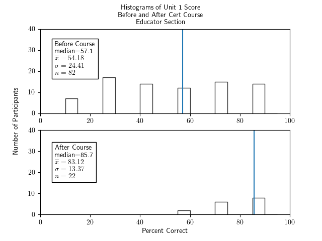
 
   Two histograms of percentage correct of the unit 1 portion of the test for participants in the educator section only - one histogram for before the course and one for after. The histogram for before the course has bars of similar heights in the low 10s from 10-15 through to 85-90, a median of 57.1, an x-bar of 54.18, a sigma of 24.41, and an n of 83.  The histogram for after the course has bars growing nearly linearly from very short at 55-60 to highest of around 8 at 85-90, a median of 85.7, x-bar=83.12, sigma=13.37, and n=22.

./make_graphs.py --prepostall --ed --ylim 40 --unit 1

Unit 1 Score, Librarian Sections Only, Pre- and Post-Test:
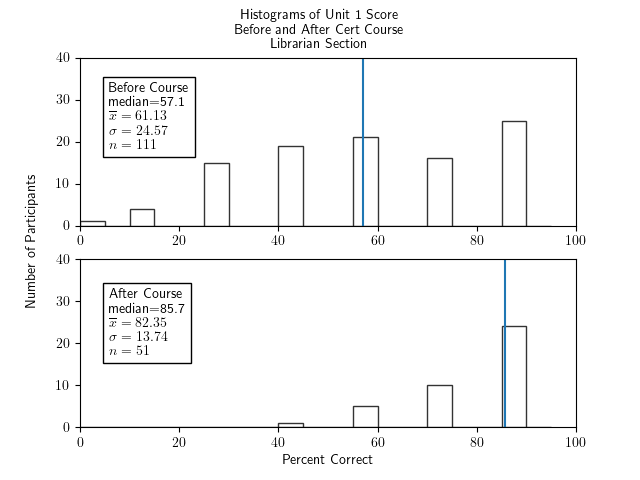
 
   Two histograms of percentage correct of the unit 1 portion of the test for participants in the librarian section only - one histogram for before the course and one for after.  The histogram for before the course has bars of similar heights in the range 15-25 from 25-30 through to 85-90 and small ones at 0-5 and 10-15, a median of 57.1, an x-bar of 61.35, a sigma of 24.57, and an n of 111.  The histogram for after the course has bars growing nearly linearly from very short at 40-45 to highest of around 25 at 85-90, a median of 85.7, x-bar=82.35, sigma=13.74, and n=51.

./make_graphs.py --prepostall --lib --ylim 40 --unit 1

Unit 1 Score, GLAM Sections Only, Pre- and Post-Test:
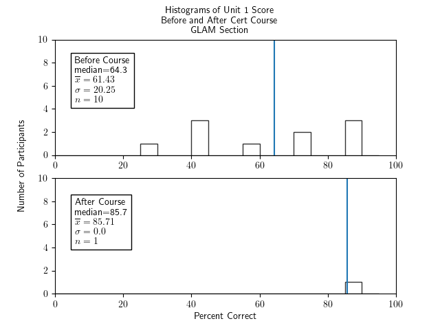
 
   Two histograms of percentage correct of the unit 1 portion of the test for participants in the GLAM section only - one histogram for before the course and one for after. The histogram for before the course has bars of similar heights of around 2 from 25-30 through to 85-90, a median of 64.3, an x-bar of 61.43, a sigma of 20.25, and an n of 10.  The histogram for after the course has one bar of height 1 at 85-90, a median of 85.7, x-bar=85.71, sigma=0, and n=1.

./make_graphs.py --prepostall --glam --ylim 10 --unit 1

Unit 2: Copyright Law

15 of the 60 survey points, or 25%, were on material from Unit 2.

Unit 2 Score, All Participants, Pre- and Post-Test:
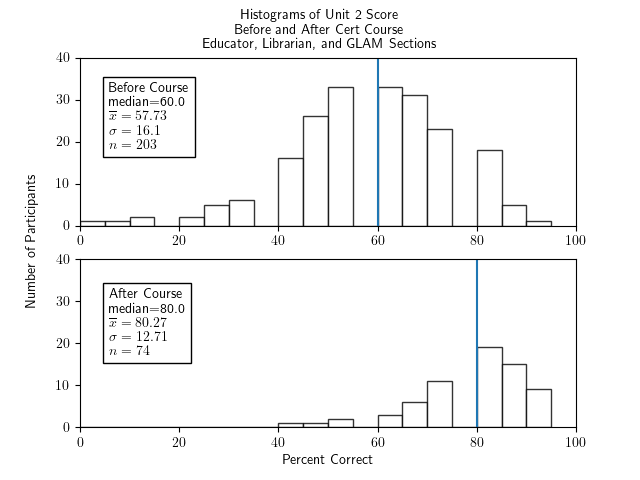
 
   Two histograms of percentage correct of the unit 2 portion of the test for all cert participants - Librarian, Educator, and section - one histogram for before the course and one for after.  Both show fairly symmetric and roughly bell-shaped distributions.  The histogram for before the course has a median of 55.0, an x-bar of 53.24, a sigma of 14.28, and an n of 203.  The histogram for after the course has a median of 77.5, x-bar=76.96, sigma=9.86, and n=74.

./make_graphs.py --prepostall --allsections --ylim 40 --unit 2

Unit 2 Score, Educator Sections Only, Pre- and Post-Test:
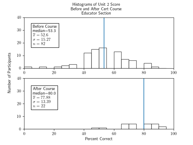
 
   Two histograms of percentage correct of the unit 2 portion of the test for participants in the educator section only - one histogram for before the course and one for after.  Both show fairly symmetric and roughly bell-shaped distributions.  The histogram for before the course has a median of 53.3, an x-bar of 52.6, a sigma of 15.27, and an n of 82.  The histogram for after the course has a median of 80.0, x-bar=77.88, sigma=13.39, and n=22.

./make_graphs.py --prepostall --ed --ylim 40 --unit 2

Unit 2 Score, Librarian Sections Only, Pre- and Post-Test:
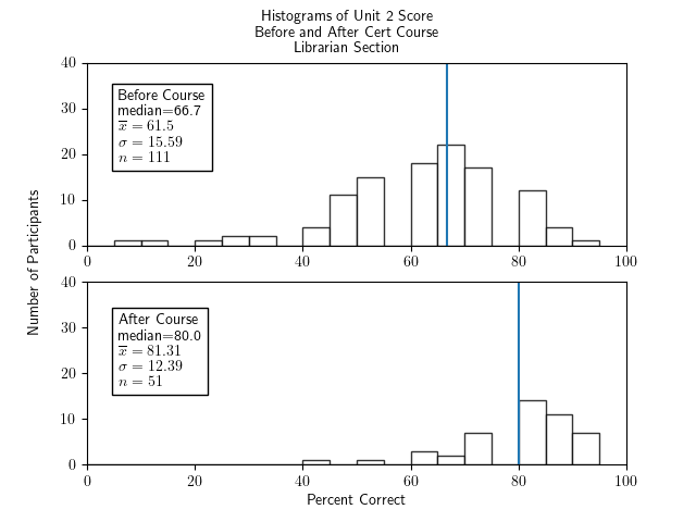
 
   Two histograms of percentage correct of the unit 2 portion of the test for participants in the librarian section only - one histogram for before the course and one for after.  Both show fairly symmetric and roughly bell-shaped distributions.  The histogram for before the course has a median of 66.7, an x-bar of 61.5, a sigma of 15.59, and an n of 111.  The histogram for after the course has a median of 80.0, x-bar=81.31, sigma=12.39, and n=51.

./make_graphs.py --prepostall --lib --ylim 40 --unit 2

Unit 2 Score, GLAM Sections Only, Pre- and Post-Test:
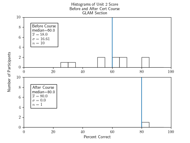
 
   Two histograms of percentage correct of the unit 2 portion of the test for participants in the GLAM section only - one histogram for before the course and one for after. The histogram for before the course has bars of similar heights of around 2 from 25-30 through to 85-90, a median of 60.0, an x-bar of 58.0, a sigma of 16.61, and an n of 10.  The histogram for after the course has one bar of height 1 at 85-90, a median of 80.0, x-bar=80.0, sigma=0, and n=1.

./make_graphs.py --prepostall --glam --ylim 10 --unit 2

Unit 3: Anatomy of a CC License

13 of the 60 survey points, or 21.6%, were on material from Unit 3.

Unit 3 Score, All Participants, Pre- and Post-Test:
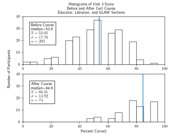
 
   Two histograms of percentage correct of the unit 3 portion of the test for all cert participants - Librarian, Educator, and section - one histogram for before the course and one for after. The histogram for before the course shows a fairly symmetric and roughly bell-shaped distribution with a median of 53.8, an x-bar of 52.03, a sigma of 17.76, and an n of 203.  The histogram for after the course has a more random shape with two low groups of bars in the range 45-70 and three higher bars in the range 75 to 95, with a median of 84.6, x-bar=80.35, sigma=13.92, and n=74.

./make_graphs.py --prepostall --allsections --ylim 40 --unit 3

Unit 3 Score, Educator Sections Only, Pre- and Post-Test:
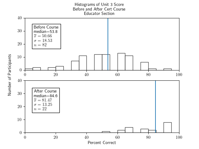
 
   Two histograms of percentage correct of the unit 3 portion of the test for participants in the educator section only - one histogram for before the course and one for after. The histogram for before the course shows a fairly symmetric and roughly bell-shaped distribution with a median of 53.8, an x-bar of 50.66, a sigma of 18.53, and an n of 82.  The histogram for after the course has a more random shape with some bars in the range 50-85 of height 3-5 and a higher bar at 90-95 of height 7, with a median of 84.6, x-bar=81.47, sigma=13.25, and n=22.

./make_graphs.py --prepostall --ed --ylim 40 --unit 3

Unit 3 Score, Librarian Sections Only, Pre- and Post-Test:
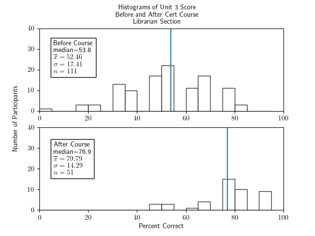
 
   Two histograms of percentage correct of the unit 3 portion of the test for participants in the librarian section only - one histogram for before the course and one for after. The histogram for before the course shows a fairly symmetric and roughly bell-shaped distribution with a median of 53.8, an x-bar of 52.45, a sigma of 17.41, and an n of 111.  The histogram for after the course has a more random shape with two low groups of bars in the range 45-70 and three higher bars in the range 75 to 95, with a median of 76.9, x-bar=79.79, sigma=14.29, and n=51.

./make_graphs.py --prepostall --lib --ylim 40 --unit 3

Unit 3 Score, GLAM Sections Only, Pre- and Post-Test:
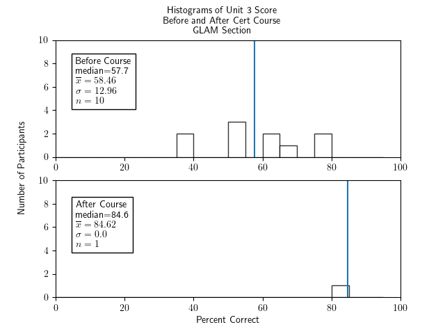
 
   Two histograms of percentage correct of the unit 3 portion of the test for participants in the GLAM section only - one histogram for before the course and one for after.  The histogram for before the course has bars of random heights of around 2 from 35-40 through to 75-80, a median of 57.7, an x-bar of 58.46, a sigma of 12.96, and an n of 10.  The histogram for after the course has one bar of height 1 at 80-85, a median of 84.6, x-bar=84.62, sigma=0, and n=1.

./make_graphs.py --prepostall --glam --ylim 10 --unit 3

Unit 4: Using CC Licenses and CC-Licensed Works

14 of the 60 survey points, or 23.3%, were on material from Unit 4.

Unit 4 Score, All Participants, Pre- and Post-Test:
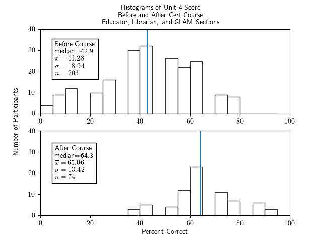
 
   Two histograms of percentage correct of the unit 4 portion of the test for all cert participants - Librarian, Educator, and section - one histogram for before the course and one for after.  Both show fairly symmetric and roughly bell-shaped distributions.  The histogram for before the course has a median of 42.9, an x-bar of 43.28, a sigma of 18.94, and an n of 203.  The histogram for after the course has a median of 64.3, x-bar=65.06, sigma=13.42, and n=74.

./make_graphs.py --prepostall --allsections --ylim 40 --unit 4

Unit 4 Score, Educator Sections Only, Pre- and Post-Test:
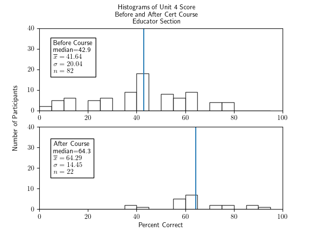
 
   Two histograms of percentage correct of the unit 4 portion of the test for participants in the educator section only - one histogram for before the course and one for after. The histogram for before the course shows a very roughly bell-shaped distribution with a median of 42.9, an x-bar of 41.64, a sigma of 20.04, and an n of 82.  The histogram for after the course has a more random shape with some bars in the range 35-45 and 70-95 of height 2-4 and a higher pair of bars at 55-65 of height 5 and 6, with a median of 64.3, x-bar=64.29, sigma=14.45, and n=22.

./make_graphs.py --prepostall --ed --ylim 40 --unit 4

Unit 4 Score, Librarian Sections Only, Pre- and Post-Test:
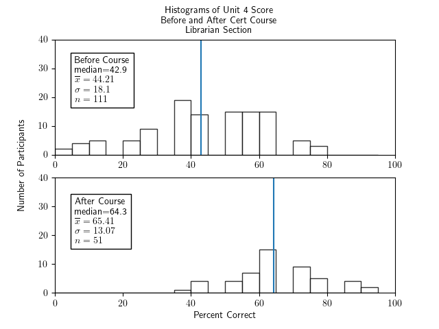
 
   Two histograms of percentage correct of the unit 4 portion of the test for participants in the librarian section only - one histogram for before the course and one for after.  Both show fairly symmetric and roughly bell-shaped distributions.  The histogram for before the course has a median of 42.9, an x-bar of 44.21, a sigma of 18.1, and an n of 11.  The histogram for after the course has a median of 64.3, x-bar=65.41, sigma=13.07, and n=51.

./make_graphs.py --prepostall --lib --ylim 40 --unit 4

Unit 4 Score, GLAM Sections Only, Pre- and Post-Test:
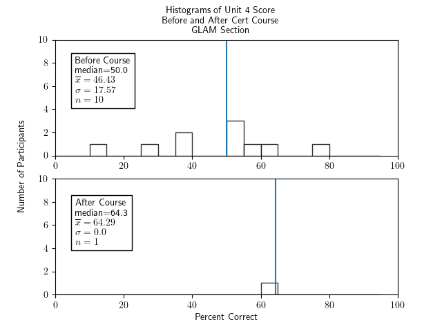
 
   Two histograms of percentage correct of the unit 4 portion of the test for participants in the GLAM section only - one histogram for before the course and one for after. The histogram for before the course shows a very roughly bell-shaped and sparse distribution with a median of 50.0, an x-bar of 46.43, a sigma of 17.57, and an n of 10.  The histogram for after the course has one bar in the range 60-65 of height 1, with a median of 64.3, x-bar=64.29, sigma=0, and n=1.

./make_graphs.py --prepostall --glam --ylim 10 --unit 4

Unit 5: CC for Educators/Librarians/GLAM

11 of the 60 survey points, or 18.3%, were on material from Unit 5.

Unit 5 Score, All Participants, Pre- and Post-Test:
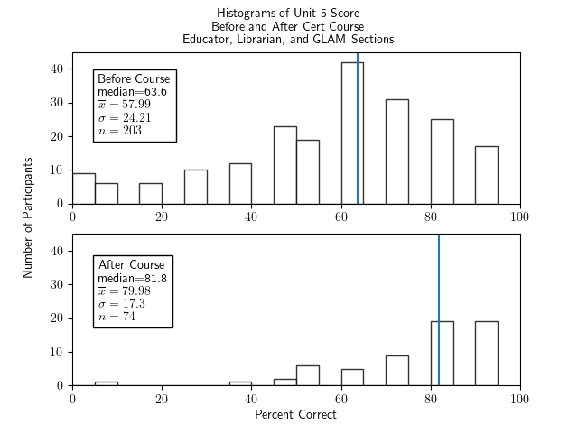
 
   Two histograms of percentage correct of the unit 5 portion of the test for all cert participants - Librarian, Educator, and section - one histogram for before the course and one for after. The histogram for before the course shows a very roughly bell-shaped and sparse distribution with a bit of a tail and bump down near 0-10, a median of 63.6, an x-bar of 57.99, a sigma of 24.21, and an n of 203.  The histogram for after the course has an outlier at 5-10, some low bars in the range 35-75 of height around 5 and two higher bars at 80-85 and 90-95 of height 18, with a median of 81.8, x-bar=79.98, sigma=17.3, and n=74.

./make_graphs.py --prepostall --allsections --ylim 45 --unit 5

Unit 5 Score, Educator Sections Only, Pre- and Post-Test:
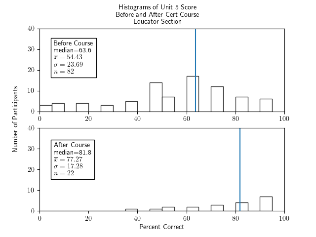
 
   Two histograms of percentage correct of the unit 5 portion of the test for participants in the educator section only - one histogram for before the course and one for after.  The histogram for before the course shows a very roughly bell-shaped and sparse distribution with a bit of a tail down to 0, a median of 63.6, an x-bar of 54.43, a sigma of 23.69, and an n of 82.  The histogram for after the course is very low and sparse starting at 35-40 of height 1 through 85-90 of height 6, with a median of 81.8, x-bar=77.27, sigma=17.28, and n=.

./make_graphs.py --prepostall --ed --ylim 40 --unit 5

Unit 5 Score, Librarian Sections Only, Pre- and Post-Test:
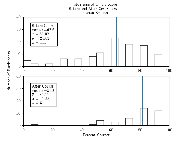
 
   Two histograms of percentage correct of the unit 5 portion of the test for participants in the librarian section only - one histogram for before the course and one for after. The histogram for before the course shows a very roughly bell-shaped and sparse distribution with a bit of a tail and bump down near 0-10, a median of 63.6, an x-bar of 61.02, a sigma of 24.02, and an n of 111.  The histogram for after the course has an outlier at 5-10, some low bars in the range 45-75 of height around 3 to 6, and two higher bars at 80-85 and 90-95 of height around 11, with a median of 81.8, x-bar=81.11, sigma=17.35, and n=51.

./make_graphs.py --prepostall --lib --ylim 40 --unit 5

Unit 5 Score, GLAM Sections Only, Pre- and Post-Test:
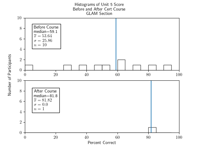
 
   Two histograms of percentage correct of the unit 5 portion of the test for participants in the GLAM section only - one histogram for before the course and one for after.  The histogram for before the course shows a scattering of bars of height 1 from 0-5 through 90-95 and one of height 2 at 60-65, with a median of 59.1, an x-bar of 53.64, a sigma of 25.86, and an n of 10.  The histogram for after the course has one bar in the range 80-85 of height 1, with a median of 81.8, x-bar=81.82, sigma=0, and n=1.

./make_graphs.py --prepostall --glam --ylim 10 --unit 5

Comparing means between units

Mean Percentage Correct In All Sections Before And After Taking The Course, By Unit:
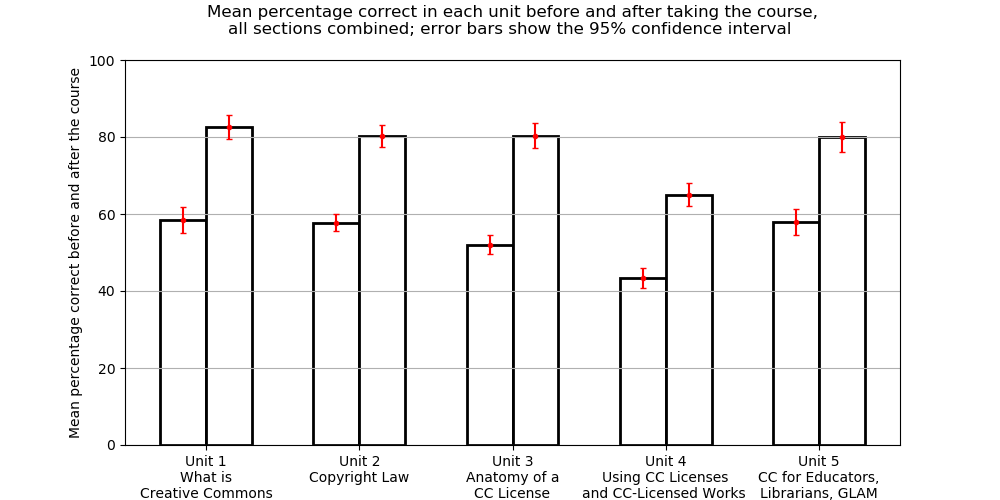
 
   Bar chart with before and after bars of percentage correct, in pairs, one pair for each unit from 1 to 5; all bars show error bars going around plus or minus five percent; in each pair, the second bar is about 20 percentage points higher than the first; the pairs all have the before bar being around 60 and after being around 80 except the Unit 4 bars which are about 10 percentage points lower.

Mean Percentage Correct in Educator Sections Before And After Taking The Course, By Unit:
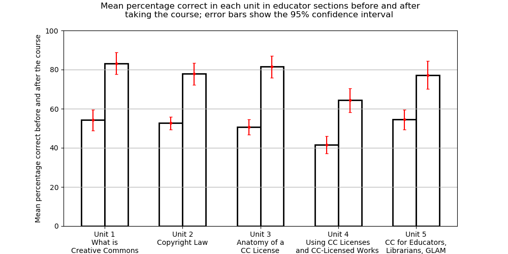
 
   Bar chart with before and after bars of percentage correct, in pairs, one pair for each unit from 1 to 5; all bars show error bars going around plus or minus five percent; in each pair, the second bar is about 20 percentage points higher than the first; the pairs all have the before bar being around 60 and after being around 80 except the Unit 4 bars which are about 10 percentage points lower.

Mean Percentage Correct in Librarian Sections Before And After Taking The Course, By Unit:
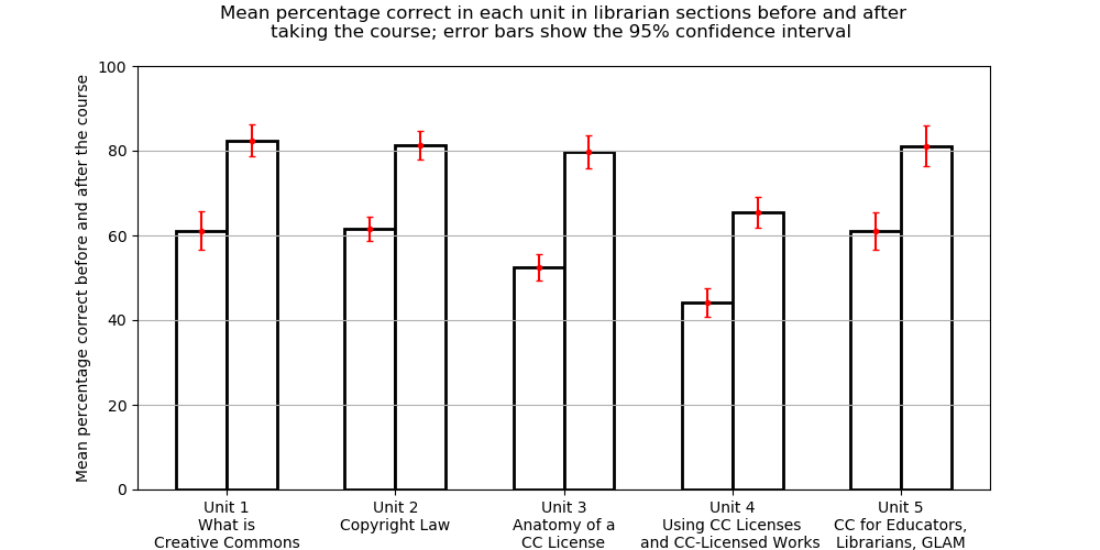
 
   Bar chart with before and after bars of percentage correct, in pairs, one pair for each unit from 1 to 5; all bars show error bars going around plus or minus five percent; in each pair, the second bar is about 20 percentage points higher than the first; the pairs all have the before bar being around 60 and after being around 80 except the Unit 4 bars which are about 10 percentage points lower.

Notes:

  1. We didn't bother to make the graphs for the GLAM students only, since there were not enough GLAM students who took the test after completing the course.
  2. For notes on how these graphs were made, see below, in the section How were these graphs made?
  3. A stats refresher for the "95% confidence interval" mentioned in each graph title: If the subset of students who took the test were a random sample of the students — which it certainly wasn't, but this kind of thing is a standard assumption in applied statistics — then the sample mean would vary a bit every time a new random sample was chosen from among all students. The 95% confidence interval is a range of values within which we would expect to see 95% of those sample means if we were repeatedly to do random samples and recalculate the sample mean each time.

Conclusions to be drawn from these disaggregations

Some things we might learn from all of these histograms:

  1. We don't have enough data from GLAM section participants to draw any reliable conclusions about those folks. Maybe we should try to get more data from this group?
  2. There is some variability between ed and lib groups in their pre-course knowledge -- e.g., librarians know a fair bit more about copyright than do educators (unsurprisingly) -- but the post-course scores tend to be quite similar, within each unit, between student groups. This would seem to indicate that we are succeeding in getting folks to the same level of knowledge about the different topics, regardless of their background.
  3. This is some variability in how successful the course graduates tend to be, by unit. In particular, we seem to bring most graduates to a score of around 85 on Units 1 and 3, a score of around 80 on Units 2 and 5, and a score of around 65 on Unit 4. Perhaps this suggests targets for where the course should put more emphasis or seek more innovative and hopefully more effective instructional approaches, in the future. -- Not that any of those scores are bad, we should say, but it would be better to have Units 2, 5, and especially 4, brought up to the very high level which is achieved for Units 1 and 3.

As long as we are thinking about what we can learn for the future from these histograms, it seems like it would be very worthwhile to do another survey of folks who finished the course some time ago, with an eye to seeing how durable is the learning that they did in the course.

How were these graphs made?

The core course content survey is a Google Form. From that form, we extract all of the results as a CSV.

If desired and possible, an extra column can be added to that CSV file, at column FW (i.e., the 179th column, or the column with Python index 178) which has either a P, F, or <anything else>, to indicated that the participant who did that survey instance either eventually passed the course, failed the course, or had unknown final status, respectively.

On a Linux box with Python 3 and lots of nice libraries, we run the script make_graphs.py and whatever options we desire.

Here is what happens if you run make_graphs.py and ask it for help:

% ./make_graphs.py --help
usage: make_graphs.py [-h] [--input_file INPUT_FILE] [--up | --uf] [--prepostpass]
                      [--prepostall] [--pretestpassfail] [--unit {1,2,3,4,5}]
                      [--ylim YLIM] [--ed] [--lib] [--glam] [--allsections]

Make graphs associated with pre- and post-test of material in the Creative Commons
Certificate coures.

optional arguments:
  -h, --help            show this help message and exit
  --input_file INPUT_FILE
                        CSV file that contains test results as produced by Google Forms,
                        based on the test dating 17 Jan 2022, but including a column FW
                        (i.e., column with Python list index 178) put in by hand that
                        indicates P or F or <anything else> depending upon whether that
                        participant eventually passed, failed, or their final status is
                        unknown. Default is 'results.csv'.
  --up                  treat participants whose pass/fail status in the course is
                        unknown as if they passed (conflicts with '--uf')
  --uf                  treat participants whose pass/fail status in the course is
                        unknown as if they failed (conflicts with '--up')
  --prepostpass         show paired graphs of pre- and post-scores, for only passing
                        folks
  --prepostall          show paired graphs of pre- and post-scores, for all students
                        (P&F)
  --pretestpassfail     show paired graphs of pass vs fail students on pre-tests
  --unit {1,2,3,4,5}    consider only the score for parts of test corresponding to the
                        specified unit of the course; when missing, use the entire test
                        score
  --ylim YLIM           the upper limit of y-axes of the histograms; when absent, picks
                        automatically
  --ed                  show graphs for educator section participants
  --lib                 show graphs for librarian section participants
  --glam                show graphs for GLAM section participants
  --allsections         show graphs which combine participants from all sections (ed,
                        lib, and GLAM)


N.B.:

  1. Multiple graphs can be produced, by selecting the appropriate options — or none at all will be made without any options. Execution pauses on each graph and users may click on the appropriate icon in the matplotlib window to save the graph as a .png. When that graph window is then closed, execution will continue, possibly making more graphs in the same way.
  2. make_graphs.py is openly licensed (of course!) under the GPLv3.


The graphs of unit-level before and after means and confidence intervals in the above section Unit-level performance were all made with the single (openly licensed, of course) script compare_units.py which has the means and standard deviations computed by make_graphs.py hard-coded in. So if you want to do this again in the future with new data, you'll have to either have to hard-code in new numbers or make a new script compare_units.py.

Conclusion

First of all, thank you, if you've made it all the way here! Many people are driven off by a statistical chart or term! Stephen Hawking was told that every equation in a popular science book he was writing would reduce the readership by an additional half &mdash: I bet there is something like this for every statistical chart or mention of a technical statistical term. And there are so very many stats charts and terms in the above text...

Second of all, the big conclusion is pretty clear and quite positive:

There is very robust knowledge gain in this course, with folks starting out at a solid F (mean of 53%) before the course (not surprisingly: why should folks know something before they study it?) and ending at B- (mean of 80%), with many Bs and even As.
Additionally, the unit-level disaggregation shows we are very doing well in our instruction across topics in the course, although there is a good target for improvement (bringing the post-course scores up by about 10%, more into line with the other units).

The approach to studying how effective is a course (or professional developement opportunity) is one that I have not seen done so carefully and completely elsewhere. I wonder if it would make sense to do so, e.g., in a multi-section version of some standard course in higher ed (like intro to calculus or anatomy and physiology).

One last thing I would like to do by way of tracking the efficacy of a course, but which we have not yet done even here, would be to get some group of folks to take the test an additional time, some months or even a year or more after they completed the course. This would give us some information on the durability of the knowledge acquired in the course ... something which is rarely studied in pedagogy (that I have seen), but which is our actual, ultimate goal in teaching.