Colorado State University — Pueblo; Fall 2016
Math 156, Introduction to Statistics
Correlation and Linear Regression
The below is a brief discussion of the work we do in this class with bivariate
data [data which has two variables about the same population]. These
explanations are shorter and the formulæ easier to use than in our book,
but below there are essentially no examples so the book is still useful.
So suppose we have some population about which we are interested in two
quantitative variables. We pick one of them to be the independent or
explanatory variable, which we write $X$, and we then call the other
the dependent or response variable, which we write $Y$.
Scatterplots
Given such a population and RVs $X$ and $Y$, we make a scatterplot by
putting a dot on a piece of graph paper at the location $(x,y)$ for each
individual in the population whose with those values of the RVs.
Well-made scatterplots ...
- have one dot for each individual in the population (although if some of
those dots overlap each other, it might look like it has fewer),
- have labels on their axes telling what the variables are and what
are the units for those variables, and
- have a few numbered tick-marks on their axes enabling the viewer to figure
out the numerical values of the coordinates of the dots in the graph.
Qualitative description of scatterplots
Looking at a scatterplot, we immediately can make a guess as to whether the
relationship behind the picture is deterministic or exhibits (some)
randomness, by seeing if there is a clear pattern (deterministic),
or a clear pattern from which there is, however, some small, apparently random
deviations (some randomness), or if the data is just scattered all over
the place (completely random).
We also frequently describe three basic features of a scatterplot:
- Shape: Does the pictured relationship have at least some apparent
determinism and, if so, what is the pattern is seems to have? Descriptive
words we might use here are linear and non-linear/curved, the
latter sometimes being refined to parabolic, exponential,
etc.
- Strength: If the scatterplot has some apparent shape, but there
is a fair bit of randomness around that shape, we say the association is
weak, while if there is very little randomness, so the scattering
of data point lies very close to the curve described by the shape
you suspect underlies the association, we call it strong.
- Direction: If there is a fairly strong association, particularly
if it is linear, we call it positive if it is increasing (in the
sense that as $x$ increases, so does $y$), while we say it is
negative if it is decreasing (in the sense that as $x$ increases,
$y$ decreases).
Quantitative description of scatterplots
Just as happened with 1-variable statistics, with bivariate data we have
quantitative measures that are more precise — although they have some
limitations — than just the qualitative descriptions above. The first
of these is the correlation coefficient (which our book calls the
linear correlation coefficient, although it is actually more common to
call it the Pearson correlation coefficient, named after its inventor
Karl Pearson). For a dataset of size $n$ with values
$(x_1,y_1),\dots,(x_n,y_n)$, the correlation coefficient is given by
$$r=\frac{1}{n-1}\sum\left(\frac{x_i - \overline{x}}{S_x}\right)\left(\frac{y_i - \overline{y}}{S_y}\right)\ .$$
Here $\overline{x}$ is the mean, and $S_x$ is the standard deviation, of the $x$
values, and likewise $\overline{y}$ is the mean, and $S_y$ is the standard
deviation, of the $y$ values.
The correlation coefficient has the following properties:
- It's always in the range from $-1$ to $1$: $-1≤r≤1$.
- It has no units (since the $x_i$, $\overline{x}$, and $S_x$ all have the
same units, and likewise for the $y$'s, so the units cancel out in the
above expression for $r$). This is good, it means that if you change the
units you use for measurements, such as from feet to meters, the
correlation coefficient doesn't change.
- The sign ($\pm$) of $r$ indicates the direction of the association
in the scatterplot: $r<0$ means the association is negative,
$r>0$ means it is positive,
- The closer $r$ is to $\pm1$, the stronger the linear association,
while the closer it is to $0$, the weaker. However, if there is a
very strong but non-linear association, the $r$ might well be close
to $0$.
Here is a nice picture of the range of values of the correlation coefficient
and what a typical scatterplot with those values might look like [from our
textbook Introduction to Statistics produced by
Saylor Academy]:

Computing the correlation coefficient by hand is not recommended. It is
almost always far better to use a calculator or computer program or website to
do it for you. There are so many different electronic tools students use, we
will not have specific directions for all of them here: instead, go to your
favorite Internet search engine and type in
- "correlation coefficient <your device name>" (such
as, for example, "correlation coefficient TI-84"), or
- "online correlation coefficient calculator" (if you prefer to
use a smartphone or website on your laptop)
and there will generally be many tutorials for you to choose from to learn how
to use your device for this purpose. Spreadsheet programs like Excel
or LibreOffice Calc will also have
built-in correlation coefficient calculators, as does the tool your instructor
often uses in the classroom, desmos.com. (For
instructions, an Internet search is again the best way to go ... although
Desmos has a handy-dandy User Guide
here.)
<
The meaning of the square of the correlation coefficient
Since the correlation coefficient $r$ of some bivariate data always satisfies
$-1≤r≤1$ and tells that the patter of the scatterplot is quite linear,
when its value is near $\pm1$, the square of $r$ will tell us how linear the
pattern is simply by being near $1$. In fact, $r^2$ always lies in the range
$0≤r^2≤1$ and can be interpreted as a percentage:
- The square $r^2$ of the correlation coefficient tells us the percentage
of the variation of the dependent variable $y$ which is caused by
variation of the independent variable $x$.
- If the square of the correlation coefficient between the
independent variable how many hours a week a student studies
statistics and the dependent variable how many points the
student gets on the statistics final exam is $.64$, then 64% of
the variation in scores for that class is cause by variation in how
much the students study. The remaining 36% of the variation in
scores is due to other random factors like whether a student was
coming down with a cold on the day of the final, or happened to sleep
poorly the night before the final because of neighbors having a
party, or some other issues different just from studying time.
Linear Regression
Suppose we have bivariate data, we make the scatterplot, and we see there is a
strong enough linear relationship that we think something is going on behind the
data. It would be nice to have the actual equation of that line.
Background on equations of lines
Recall the equation of a line is usually in the form $y=mx+b$, where $x$ and
$y$ are variables and $m$ and $b$ are numbers. Some basic facts about lines:
- If you are given a number for $x$, you can plug it in to the equation
$y=mx+b$ to get a number for $y$, which together give you a point with
coordinates $(x,y)$ that is on the line.
- $m$ is the slope, which tells how much the line goes up (increasing
$y$) for every unit you move over to the right (increasing $x$) &mdash we
often say that the value of the slope is $m=\frac{rise}{run}$. It can be
- positive, if the line is tilted up,
- negative, if the line is tilted down,
- zero, if the line is horizontal, and
- undefined, if the line is vertical.
- $b$ is the $y$-intercept, which tells the $y$-coordinate of the
point where the line crosses the $y$-axis.
The best line: residuals
The line we are looking for to
represent some fairly strong, linear data in a scatterplot should be the best
line, in some sense. The most common meaning given to best in this
search for the line is he line whose total square error is the smallest
possible. That is, if we draw a candidate for the best line, it might
not pass directly through all of the data points, so for each data point at
location $(x_i,y_i)$, there is a point on the line with the same $x$
coordinate, but maybe with a different $y$ value, say $\widehat{y_i}$; so
$(x_i,\widehat{y_i})$ is on the line. The difference $y_i-\widehat{y_i}$ is
called the error or, more often, the residual. Here is a picture of
an example, again from our textbook
[Introduction
to Statistics produced by
Saylor Academy]:
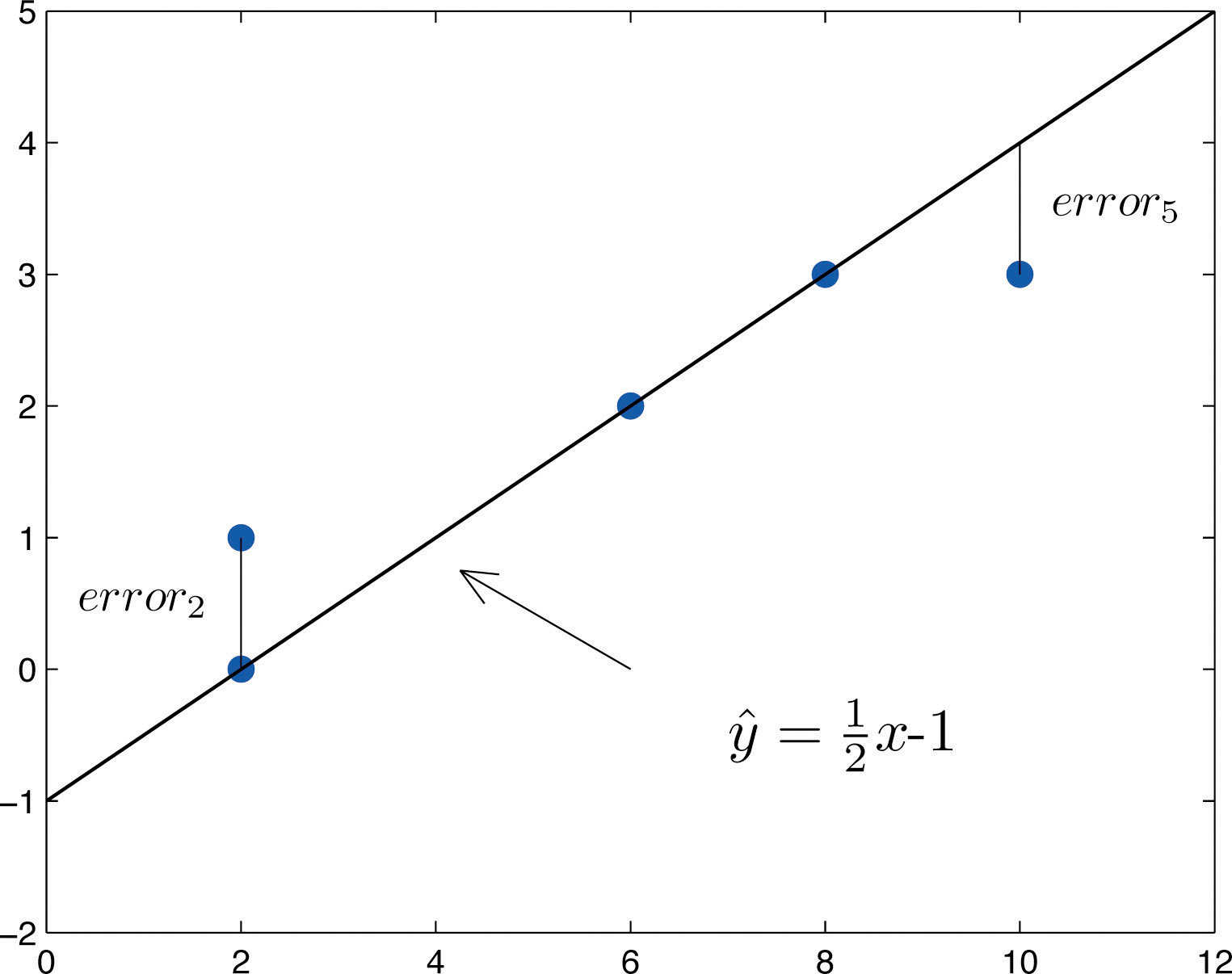
[Note the $\frac{1}{2}x-1$ is just an example — in your work, other
numbers than $\frac{1}{2}$ and $-1$ will probably be what you will use for the
slope and $y$-intercept.]
The LSRL: how to find it
The line we shall use in this kind of situation has the smallest sum of the
squares or the residuals, and is therefore called the
least squares regression line [LSRL]. Here are the important
formulæ:
$$\widehat{y} = m x +b\quad\text{where}\quad m=r\frac{S_y}{S_x}\quad\text{and}\quad b=\overline{y}-m\overline{x}\ .$$
Here of course $r$ is the correlation coefficient, $\overline{x}$ is the mean,
and $S_x$ is the standard deviation, of the $x$ values, while $\overline{y}$ is
the mean, and $S_y$ is the standard deviation, of the $y$ values. Again we are
using $\widehat{y}$ to indicate a predicted $y$-value, a value on the
LSRL, as opposed to the symbol $y$, which we will reserve for actual $y$ values
of data points.
One thing to notice about the LSRL is that it always passes through the
point $(\overline{x},\overline{y})$ whose coordinates are the means of the
$x$ values and the $y$ values, separately. This makes sense since that point
should pretty much be in the middle of the cloud of data points.
Once again, it is not recommended to compute the coefficients (the slope
and the $y$-intercept) of the LSRL by hand using the above formul&aeli;. Use
your favorite electronic tool instead, again after finding instructions by
an Internet search for "regression line <your device name>" this
time. Note that
- For the TI-8x calculators, the function you probably want to use is
called LinReg(ax+b) (and yes, the $a$ it computes here is the
slope, which we usually write $m$ while the $b$ is the same as our $b$,
being the $y$-intercept).
- In Desmos, to get the regression line for some data you have entered as
a table of data into the variables $x_1$ and $y_1$, you want to type
"$y_1 \sim m x_1 + b$" over on the left where you put in data and equations
to be graphed.
The LSRL: basic uses
One of the simplest things we do with the LSRL is to use it to predict $y$
values for some new $x$ values. That is, if we have an $x$ value for which we
do not know the corresponding $y$ — that is, $(x,y)$ is not a point in
our dataset — we can guess that the $y$ value should probably be the
$\widehat{y}$ given by the equation of the LSRL. If the $x$ we use to generate
this new guess point $(x,\widehat{y})$ is near or in amongst the known $x$
values (basically, if the new $x$ would not be an outlier for the $x$ values of
your dataset), then this process of generating a guess for the corresponding
$y$ is called interpolation.
For example, in the above example where we had $\widehat{y}=\frac{1}{2}x-1$,
if you had to guess what would have been the $y$ value for $x=2$, you would
guess the value $\frac{1}{2}2-1$, or $0$.
Another use of the LSRL is to interpret the coefficients of its equation in
the context of your data.
- The slope $m$ tells us how much the $y$ variable will increase, on
average, when the $x$ variable increases by one unit.
- For example, suppose $x$ is the number of units — often called
widgets by economists — your factory makes and $y$ is
the cost to manufacture that many widgets. Then the cost of
manufacturing each additional widget (which economists call the
marginal cost per widget) is simply the value of $m$, the
slope of the LSRL. [This cost will be made up of things like the
cost of the materials which go into the widget, the wages of the
works for their time in making that single widget, etc.]
- The $y$-intercept $b$ tells us what we should expect the value of the
dependent variable $y$ to be if the independent variable $x$ had the value
0.
- Again, suppose $x$ is the number of widgets your factory makes and
$y$ is the cost to manufacture that many widgets. Then the cost to
make no widgets at all (the fixed costs of keeping the factory
open) is $b$, the $y$-intercept of the LSRL equation. [This cost will
consist of things like the rental fee for the factory building, the
salaries of the managers who are paid even without directly contributing
to the production of each individual widget, etc.]
The LSRL: some cautions
It turns out that we have to be careful of using the LSRL. Here are some of the
ways to be careful:
- Extrapolation: Often one collects data, makes a scatterplot and
LSRL, and then wants to predict the $y$ value corresponding to an $x$
value well past the end of the $x$s in the dataset. This is considered a
very dangerous thing to do, essentially because the shape of the scatterplot
might be radically different if we were able to collect enough data to
fill all the way out to where the new, interesting $x$ is. That would mean
that the equation of the LSRL would be quite different, so to use the LSRL
equation we have with just the small dataset would be foolish. It is
something we worry enough about to give it a name, extrapolation,
and statistics texts repeatedly warn not to do it.
[It must be admitted, though, that sometimes extrapolation is the only
thing you can do, and so gives the best guess for what the
interesting $y$ will be. There is a famous example of this in which the
engineers at the company Morton Thiokol recommended, the night before a
scheduled launch of the space shuttle Challenger, that the
launch be delayed, because an extrapolation of the scatterplot showing
number of O-ring burn-throughs versus launch temperature,
plus the forecast temperature for the next day, indicated that there
would be a dangerous number of these burn-throughs. Managers ignored this
warning, and the Challenger did in fact blow up the next
day. It was extrapolation, but it was a good guess.]
- Outliers: All of the formulæ above for $r$, $m$, and $b$
are built using means and standard deviations that we know are sensitive
to outliers. So if even a single additional data point is added to a
dataset which has quite different values from the rest, it can change the
LSRL quite a bit. In short,
- The LSRL is very sensitive to outliers.
Of course, what is an outlier is a little more subtle for bivariate data:
it is a value of $(x,y)$ which is far away from the general trend of the
other data. In particular, a point on a scatterplot might have an $x$
coordinate which is not an outlier, looking just at the $x$ values, and
a $y$ coordinate which is not an outlier just among the $y$ values, but
nevertheless be an outlier in the scatterplot if it is far away from the
general trend of the rest of the data.
- Patterns in the residuals: The residuals, which are the errors
of the LSRL in matching the actual data, should not have any particular
pattern or shape. So if you graph them, it should be a random picture which
you would say is entirely random. If, instead, the graph of the residuals
has some over-all shape, that probably indicates that the LSRL was not a
good tool to study the original data, because it probably had a general
shape which was not actually linear.
It is for this reason that many electronic tools (e.g., Desmos)
give you the option of graphing the residuals to look for that possible
pattern.
- Causation: When you collect data, find a strong association,
make useful interpolations (and maybe even extrapolations) with the LSRL,
it is easy to think that this is all going so well because the values of
the independent variable $x$ are causing the dependent variable $y$
to take its corresponding values. But, in fact, all you have found is
association, not causation. They might be associated because
of some other lurking factor, or even the causal arrow might go in the
other direction, and you would not be able to tell just by this work with
scatterplots, correlation coefficients, and LSRLs. We often summarize this
by saying
Correlation is not causation.
and this is indeed a good think to keep in mind.
- For example, there is a famously strong positive correlation between
the independent variable ice cream sales on particular days in big
American cities and the dependent variable petty crime rate on
those dates in those cities. This is not because ice cream
causes crime! Rather, they are both correlated with another, lurking
variable, temperature: on nice, warm days, people buy ice cream
and (probably other people) commit small crimes. On cold, winter days,
no one is outside either to buy ice cream or to commit crime.
- We should also be aware that while correlation is not causation,
it sure is a hint. So we should not entirely reject the
causal evidence of strong correlation, just use it with care.